Lagrange Points

Introduction

The Lagrange Points are equilibrium points in a dynamic system. They are positions in space among the Three-Body Problem where the third body is in gravitational force equilibrium with respect to \(P_1\) and \(P_2\). These regions in space are often considered in spacecraft mission design as they require little to no energy to maintain position. Some spacecraft missions have made use of operating at Lagrangian Points. The ESA/NASA Solar and Heliospheric Observatory Satellite (SOHO) spacecraft moves around the Sun with Earth at Lagrange Point 1 for the Sun-Earth system. There SOHO is locked in place with an uninterrupted view of the Sun and continues to study the structure and dynamics of the Sun. On the other hand Lagrange Point 2 is ideal for astronomy research as it is keeps the Sun, Earth and Moon behind the spacecraft and provides a view of deep space for telescopes. Lagrange Point 2 was previously the home of the ESA operated space telescope Planck from 2009-2013 were it aimed to observe the Cosmic Microwave Background at microwave and infrared frequencies. Currently Lagrange Point 2 is home to the James Webb Space Telescope, an infrared observatory looking back to towards the beginning of time.

This section will provide an overview of how to define and analyze the Lagrangian Points for a dynamical system in the Non-Dimensional Circular Restricted Three-Body Problem (CR3BP).

More on the stability of Lagrange Points in the next section Stability of Equilibrium Points.

---

From previous section on the CR3BP, the potential for this system is defined as (7):

(1)\[\tilde{V}\left(x^*,y^*,z^*\right) = \frac{1}{2}\left( {x^*}^2 + {y^*}^2\right) + \frac{1-\mu}{r^*_1} + \frac{\mu}{r^*_2}\]

where \(r^*_1\) and \(r^*_2\) are:

(2)\[\begin{split}\begin{align*} r^*_1 &= \sqrt{\left( x^* + \mu \right)^2+{y^*}^2+{z^*}^2} \\ r^*_2 &= \sqrt{\left( x^* - 1 + \mu \right)^2+{y^*}^2+{z^*}^2} \end{align*}\end{split}\]

Warning

The non-dimensional length term in section Non-Dimensional Circular Restricted Three-Body Problem is defined as:

\[\mathbf{r}^* = \frac{\mathbf{r}}{r_s} = \frac{\mathbf{r}}{R}\]

For this section on Lagrange Points & Stability, use of notation \(^*\) will be dropped from Non-Dimensional state parameters.

To find the location of the Lagrange Points take the partial derivative of \(\mathbf{\tilde{V}}\) and find locations where motion is zero. Taking the partial of \(\mathbf{\tilde{V}}\) (1) yields:

(3)\[\begin{split}\begin{align*} \frac{\partial{\mathbf{\tilde{V}}}}{\partial{x}} &= x - \frac{(1-\mu)(x+\mu)}{{r_1}^3} - \frac{\mu(x+\mu-1)}{{r_2}^3} \\ \frac{\partial{\mathbf{\tilde{V}}}}{\partial{y}} &= \left[ 1 -\frac{1-\mu}{{r_1}^3} - \frac{\mu}{{r_2}^3} \right]y \\ \frac{\partial{\mathbf{\tilde{V}}}}{\partial{z}} &= -\left[ \frac{1-\mu}{{r_1}^3} + \frac{\mu}{{r_2}^3} \right] \end{align*}\end{split}\]

From plotting the potential there are clues about how many and where the Lagrange Points lie. Below is a screen shot of Interactive Figure 1.6 from section on Non-Dimensional Force Potential for the Non-Dimensional CR3BP.

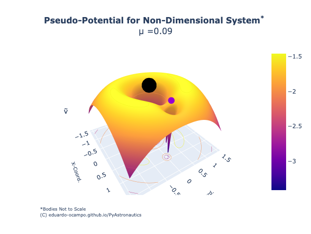
Figure 1.17 Screenshot of Non-Dimensional CR3BP Potential Plot

By looking at the pseudo-potential plot one might infer there exist equilibrium points along the saddle of the curve or somewhere along the upper rim of the surface plot. Think of it at spots on the curve where you might be able to balance a ball from rolling down.

There are known to be 5 equilibrium points (\(L_{1-5}\)) along the potential surface for a Three-Body System. \(L_{1-3}\) lie collinear along the axis joining primaries \(P_1\) and \(P_2\) while \(L_{4-5}\) lie to the side and equidistant to both bodies.

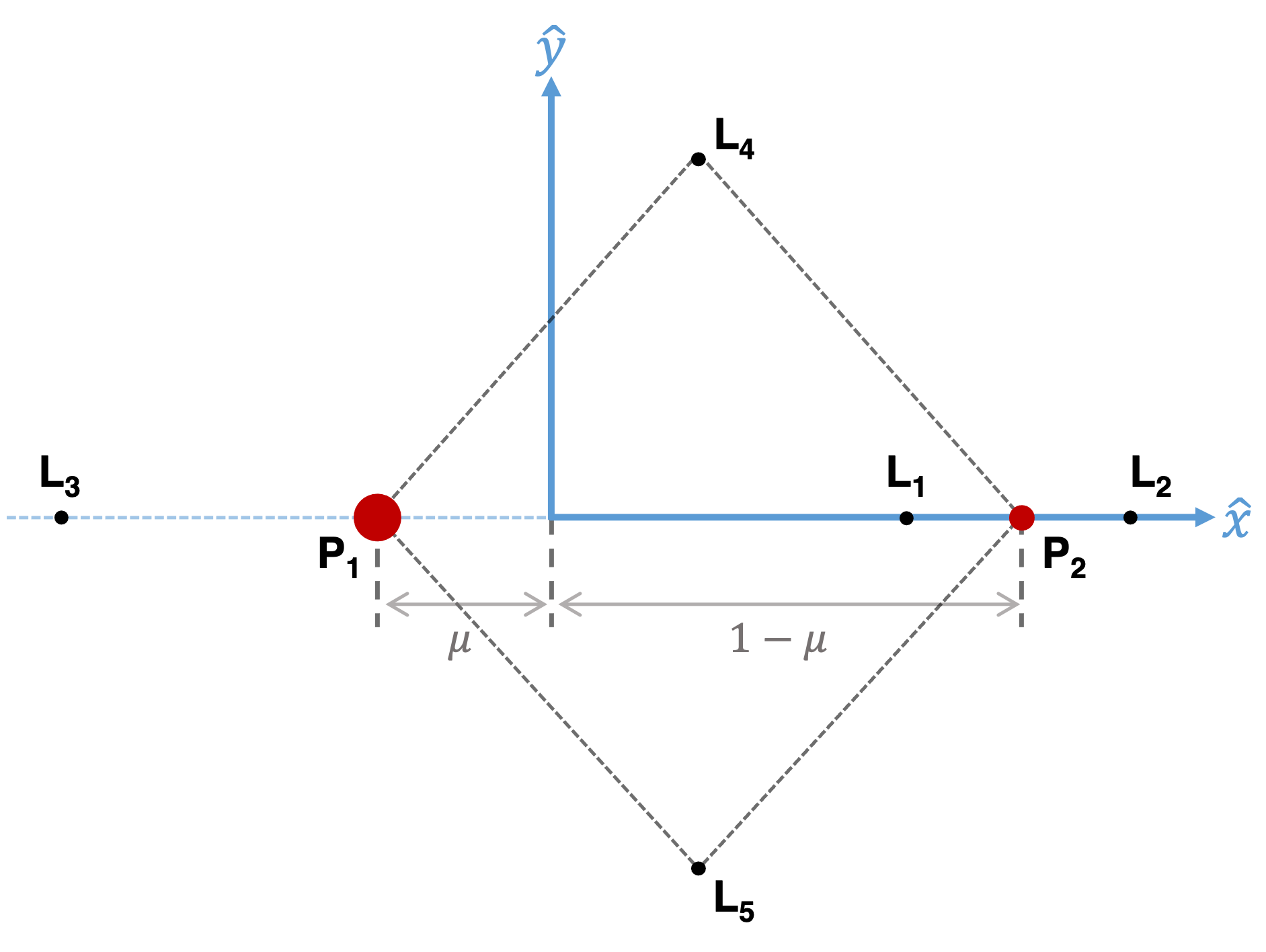
Figure 1.18 X-Y Topology of Lagrange Points in the Rotating Coordinate Frame

Collinear Lagrange Points

For the collinear Lagrange Points \(L_{1-3}\) the y- and z-coordinates are zero. This reduces their known position vectors (2) to depend only on their location along the x-axis relative to their primary bodies.

(4)\[\begin{split}\begin{align*} r_1 &= |x+\mu| \\ r_2 &= |x-1+\mu| \end{align*}\end{split}\]

To compute the x-coordinates of the collinear Lagrange Points we need to solve \(\frac{\partial{\mathbf{\tilde{V}}}}{\partial{x}}\) only since \(y = 0\) and \(z = 0\). Substitute the relative position vectors (4) into \(\frac{\partial{\mathbf{\tilde{V}}}}{\partial{x}}\) (3).

(5)\[\frac{\partial{\mathbf{\tilde{V}}}}{\partial{x}} = x - \frac{(1-\mu)(x+\mu)}{|x+\mu|^3} - \frac{\mu(x+\mu-1)}{|x-1+\mu|^3} = 0\]

By plotting \(\frac{\partial{\mathbf{\tilde{V}}}}{\partial{x}}\) we are given a quick and easy means of locating Lagrange Points \(L_{1-3}\) for an arbitrary \(\mu\).

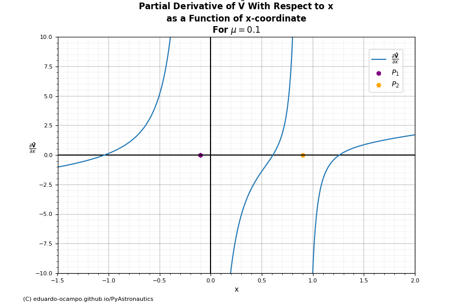
Figure 1.19

Notice the function crosses the x-axis (\(\frac{\partial{\mathbf{\tilde{V}}}}{\partial{x}}\big|_{x=0}\) ) precisely were the collinear points (\(x_{1-3}\)) lie. At the same time, \(\frac{\partial{\mathbf{\tilde{V}}}}{\partial{x}}\) heads asymptotically towards infinity at primary \(P_1\) and similarly as the x-coordinate approaches \(P_2\).

To aid in solving for the roots \(\frac{\partial{\mathbf{\tilde{V}}}}{\partial{x}}\big|_{x=0}\) it helps to approximate the collinear equilibrium points. Expanding out Expression (5) up to the first power yields:

(6)\[\begin{split}\begin{align*} x_1 &\approx 1 - \left(\frac{\mu}{3}\right)^{\frac{1}{3}} + \sigma\left(\mu^{\frac{2}{3}} \right) \\ x_2 &\approx 1 + \left(\frac{\mu}{3}\right)^{\frac{1}{3}} + \sigma\left(\mu^{\frac{2}{3}} \right) \\ x_3 &\approx -1 + \left(\frac{\sqrt(2)-1}{3}\right)\mu + \sigma\mu^2 \end{align*}\end{split}\]

By removing higher order terms, the equations reduce to:

(7)\[\begin{split}\begin{align*} x_1 &\cong 1 - \left(\frac{\mu}{3}\right)^{\frac{1}{3}} \\ x_2 &\cong 1 + \left(\frac{\mu}{3}\right)^{\frac{1}{3}} \\ x_3 &\cong -1 + \left(\frac{\sqrt(2)-1}{3}\right)\mu \end{align*}\end{split}\]

There are many numerical solvers for getting the roots of Equation (5). Approximating the collinear Lagrange Points with the help of Equations (7) can be used to initialize a solver. An example is provide in the next section.

Computing Collinear Points Using Python

Within module astrodynamics.three_body_problem there are methods for computing the Lagrange Points for a Three-Body system given a mass ratio \(\mu\). For this example let us compute the collinear Lagrange Points by numerically solving Equation (5) using Python and compare the results to Figure 1.19

Begin by importing Python class planar_lagrange_points and setting mass ratio of 0.1.

from pyastronautics.astrodynamics.three_body_problem import planar_lagrange_points

mu = 0.1

# Define class for given μ
lagrange_points =  planar_lagrange_points(mu)

Class method colinear_approximation() computes approximate solutions for the collinear points \(x_{1-3}\) using Equations (7) which serves as an initial estimate of the root. colinear_points() uses the root estimate and the Scipy Newtow-Raphson method for finding the roots of \(\frac{\partial{\mathbf{\tilde{V}}}}{\partial{x}}\).

cp_approx = lagrange_points.colinear_approximation()
cp = lagrange_points.colinear_points()

print("Approx: ",cp_approx)
print("Roots: ",cp)

Approx:  [0.589276749, 1.210723250, -1.041666667]
Roots:   [0.609035110, 1.259699832, -1.041608908]

How do the results compare to Figure 1.19? Methods colinear_approximation() and colinear_points both return \(L_{1-3}\) in that order and only their x-coordinates because it is known that \(y=0\) for collinear points. The roots are spot on with where \(\frac{\partial{\mathbf{\tilde{V}}}}{\partial{x}}\) crosses the x-axis in Figure 1.19. The approximate solution is within reasonable tolerance to the exact solution and serves as a good starting point.

Now let us compare how the solution to \(\frac{\partial{\mathbf{\tilde{V}}}}{\partial{x}}\) changes as a function of mass ratio \(\mu\). Following the same approach as example for \(\mu = 0.1\) solve \(\frac{\partial{\mathbf{\tilde{V}}}}{\partial{x}}\big|_{x=0}\) numerically to find the collinear points for values of \(\mu\) between 1e-6 and 0.5.

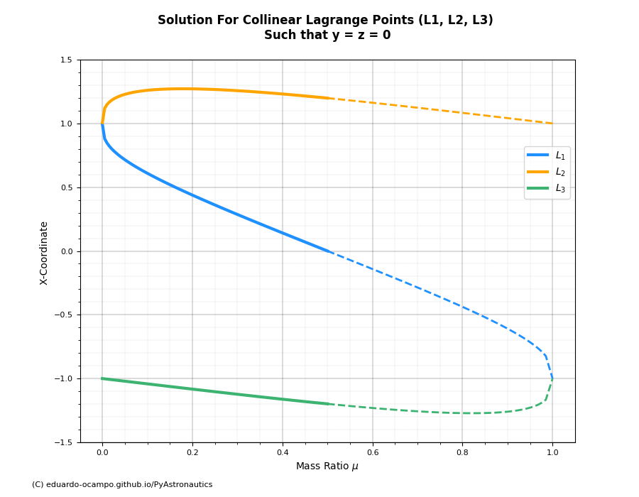
Figure 1.20

Recall from the derivation of the Non-Dimensional Equations of Motion, it assumed that \(\mu \lt \frac{1}{2}\). The dash portion of Figure 1.20 denotes solution set for when \(\mu \gt \frac{1}{2}\). It may not be obvious from looking at Figure 1.20 but the collinear points of a system for \(\mu \gt \frac{1}{2}\) is symmetric to a system where \(1-\mu\). With relative position of \(L_2\) and \(L_3\) swapping coordinates. To illustrate this consider the following example:

Let

(8)\[\begin{split}\begin{align*} \mu_1 &= \frac{m_1}{m_1+m_2} \\ \mu_1 &= 0.10 \end{align*}\end{split}\]

(9)\[\begin{split}\begin{align*} \mu_2 &= 1 - \mu_1 \\ &= 1 - \frac{m_1}{m_1+m_2} \\ &= \frac{m_2}{m_1+m_2} = 0.9 \\ \end{align*}\end{split}\]

Plot the collinear points for a Three-Body system with \(\mu_1\) and \(\mu_2\).

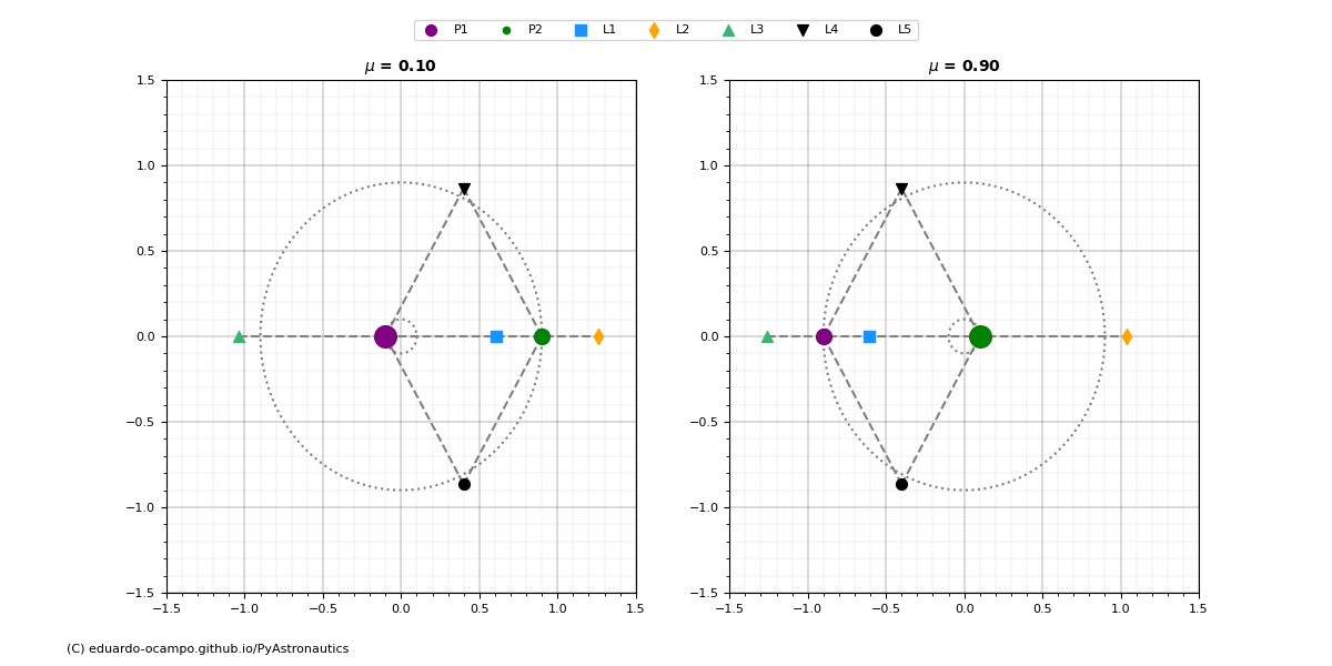
Figure 1.21 Example of Complementary Lagrange Points

Notice how the Lagrange Points for system with \(\mu_1 = 0.1\) are symmetric across the y-axis in the rotating reference frame as well as how the two masses position relative to the barycenter change.

Another interesting configuration worth mentioning is when the masses of \(P_1\) and \(P_2\) are equivalent (\(\mu = \frac{1}{2}\)). For this system \(L_1\) is position right at the barycenter, and the bodies move along the same orbit in the rotating reference frame!

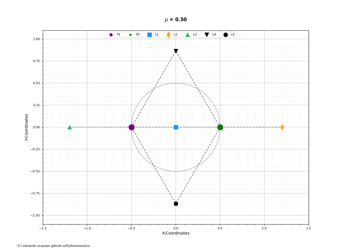
Figure 1.22 Position of Lagrange Points For Primary Bodies of The Same Mass

Lastly, here is a gif showing how the relative position of the Lagrange Points changes as a function of mass ratio:

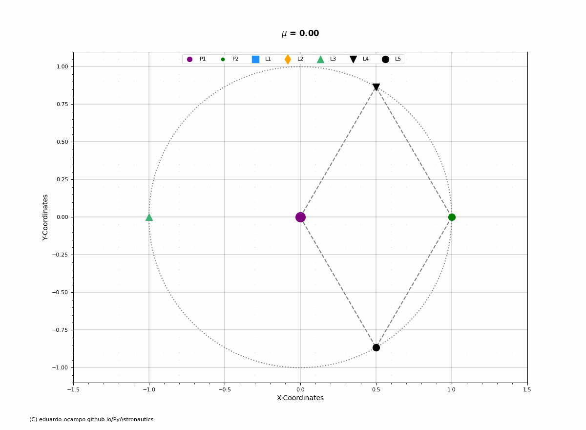
Figure 1.23 Position of Lagrange Points Within The Rotating Reference Frame

Equilateral Lagrange Points

Solving for the position of Lagrange Points \(L_{4}\) and \(L_{5}\) are fairly straightforward compared to the Collinear Lagrange Points. \(L_{4}\) and \(L_{5}\) exist such that \(y = 0\). Now check Equation (3) for \(\frac{\partial{\mathbf{\tilde{V}}}}{\partial{y}} = 0\).

\[\frac{\partial{\mathbf{\tilde{V}}}}{\partial{y}} = \left[ 1 -\frac{1-\mu}{{r_1}^3} - \frac{\mu}{{r_2}^3} \right]y = 0\]

The root for this function is trivial and results in the relative position vectors \(\mathbf{r}^3_1\) and \(\mathbf{r}^3_2\) to both be 1. Now applying this information to the definition of \(\frac{\partial{\mathbf{\tilde{V}}}}{\partial{x}}\) from Equation (3), we get:

(10)\[\frac{\partial{\mathbf{\tilde{V}}}}{\partial{x}} = x - (1-\mu)(x+\mu) - \mu(x+\mu-1)\]

Sovling for \(\frac{\partial{\mathbf{\tilde{V}}}}{\partial{x}} = 0\) gives exactly:

(11)\[x_{4,5} = \frac{1}{2} - \mu\]

and using Equation (2) from the Three-Body definition of vectors \({r_1}\) and \({r_2}\) the y-coordinates for \(L_{4-5}\) are:

(12)\[ \begin{align}\begin{aligned}y_4 = \frac{\sqrt{3}}{2}\\y_5 = -\frac{\sqrt{3}}{2}\end{aligned}\end{align} \]

These results demonstrate that Lagrange Points \(L_{4}\) and \(L_{5}\) lie equilateral with respect to primaries \(P_1\) and \(P_2\). As shown in Figure 1.18 above.

We now have the exact results of for Lagrange Points \(L_{4-5}\) whereas Lagrange Points \(L_{1-3}\) need to be solved iteratively using a root-finding soler with the aid of the approximate \(x_1\), \(x_2\) and \(x_3\) values (7).

The Lagrange Points (\(L_{1-5}\)) are fixed equilibrium points within the rotating coordinate frame. Below is an example of how the points rotate with a system (\(\mu = 0.10\)) and its angular velocity.

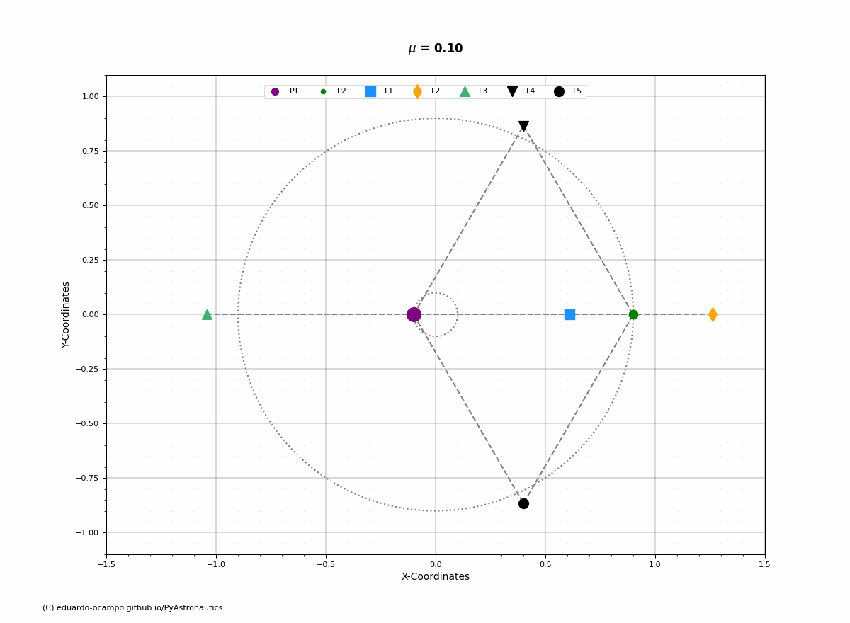
Figure 1.24 Position of Lagrange Points Within The Inertial Reference Frame

For a non-restricted Three-Body Problem system (\(\mu_3 \neq 0\)), these 5 Lagrange Points still exist. However, the positions of the collinear Lagrange Points are shifted. If the primaries \(P_1\) and \(P_2\) are on an elliptical orbit, analogue of the Lagrange Points do also exists.

Python Example

Astrodynamics module three_body_problem contains all that is needed to solve for both the collinear and equilateral Lagrange Points. Begin by initializing planar_lagrange_points with the system’s mass ratio \(\mu\). Then by calling method get_points() the scripts will numerically solve for \(L_{1-3}\) through class method colinear_points() and analytically solve for \(L_{4-5}\) through class method triangular_points(). Storing the results as attributes.

As an example let us compute the Lagrange Points for the Earth-Moon system. As defined in Jacobi Constant Python Example the Earth-Moon mass ratio is:

\[\mu = 0.012150584394709708\]

Script setup

from pyastronautics.astrodynamics import three_body_problem

# Earth-Moon System
mu = 0.012150584394709708

# Get Points
lagrange_points = three_body_problem.planar_lagrange_points(mu)
lagrange_points.get_points()

# Print L1-L5
for i in range(1,6):
    print("\nLagrange Point {}:".format(i))
    print("x = ",eval('lagrange_points.l{}x'.format(i)))
    print("y = ",eval('lagrange_points.l{}y'.format(i)))

Output

Lagrange Point 1:
x =  0.8369151317503717
y =  0

Lagrange Point 2:
x =  1.1556821607722148
y =  0

Lagrange Point 3:
x =  -1.005062645304093
y =  0

Lagrange Point 4:
x =  0.48784941560529027
y =  0.8660254037844386

Lagrange Point 5:
x =  0.48784941560529027
y =  -0.8660254037844386

Below is an interactive plot showing the Lagrange Points for the Earth-Moon system. Note that for a small mass ratio like in this example \(L_{1}\) and \(L_{2}\) lie very close the Moon. While \(L_{3,4,5}\) lie very close to the Moon’s orbital path.

Figure 1.25

References

The Lagrange Points

What is a Lagrange Point?