Introduction

The full Two-Body Problem is the motion of two bodies with finite masses that are attracted to each other according to Newton’s Law of Gravitation.

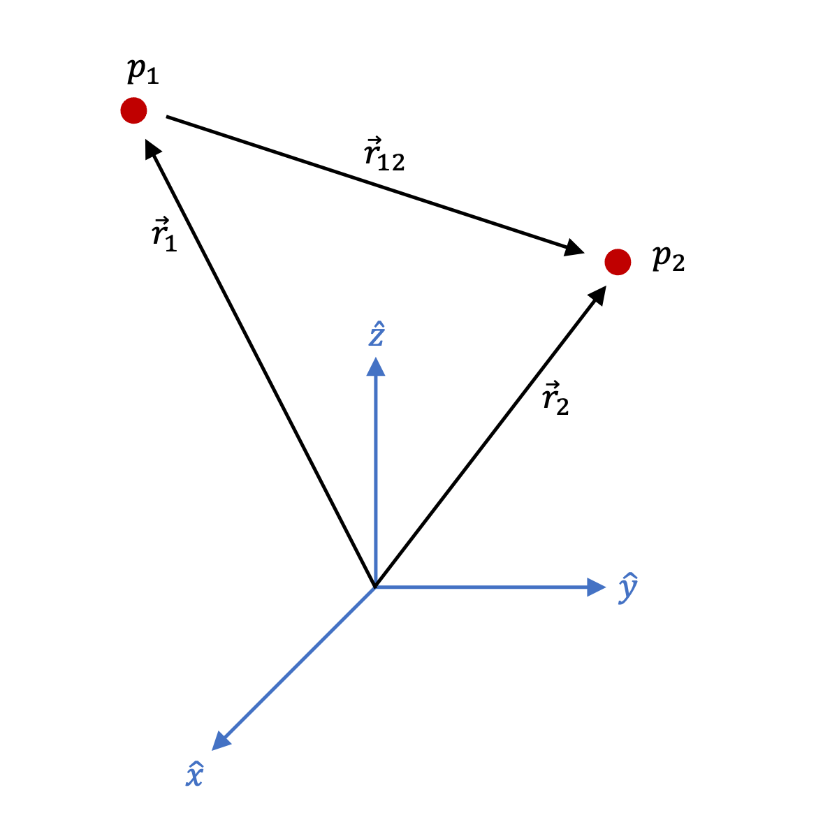
Assume we are interested in their relative dynamics. The force of particle \(P_1\) acting on particle \(P_2\) in the inertial frame yields the following diagram:

Figure 1.1 Two-Body Problem Definition in an Inertial Reference Frame

Where \(P_1\) has mass \(m_1\) and \(P_2\) has mass \(m_2\), and we define the relative vector notation as:

\[\begin{split}\begin{align*} \mathbf{r}_{ij} &= \mathbf{r}_j - \mathbf{r}_i \\ \mathbf{r}_{12} &= \mathbf{r}_2 - \mathbf{r}_1 \end{align*}\end{split}\]

Derived from Newton’s Law of Gravitation, the Equation of Motion for the Two-Body Problem is defined by Second-Order Ordinary Differential Equations:

(1)\[\ddot{\mathbf{r}} = -G\frac{(m_1+m_2)}{r^3}\mathbf{r}\]

where:

\[\mathbf{r} = \mathbf{r_{12}} = \mathbf{r_2} - \mathbf{r_1}\]

Note

The term \(G(m_1+m_2)\) comes up quite often in our Equations of Motion that is convenient to define it as the Gravitational Parameter (\(\mu\)) as the product of the Gravitational Constant (\(G\)) and Mass (\(m\)).

(2)\[\mu = G(m_1+m_2)\]

The Relative State Vector

Each particle has a State Vector made up of its position and velocity:

(3)\[\begin{split}\mathbf{x} = \begin{bmatrix} x \\ y \\ z \\ \dot{x} \\ \dot{y} \\ \dot{z} \end{bmatrix}\end{split}\]

To solve for the Two-Body Problem it requires 12 equations of motion due to 2 state vectors. However, if we assume one of the particles does not have mass or its mass is negligible (Earth-satellite system) the system will require only 6 equations of motion. Thus 6 integrals of motion are needed to solve the relative dynamics of the Two-Body Problem. The 6 integrals of motion have become to be known as the Classical Orbital Elements. An integral of motion is a combination of positions, velocities, and times that remain constant under the motion governed by the equations of motion.

For Two-Body systems were \(m_2 \ll m_1\) the Expression (2) for Gravitational Parameter simplifies to:

(4)\[\mu = G(m_1)\]

NASA JPL’s Solar System Dynamics Group maintains and publishes accurate Astrodynamic Parameters for planetary bodies. Below are just a few common gravitational parameters for planets in our Solar System. Visit Astrodynamic Parameters to find more information:

Body	GM (\(km^3s^{-2}\))
Sun	1.32712440041279e11
Earth	398600.435507
Mars	42828.375816
Saturn	137940584.841800

Solving The Two-Body Problem

As an example for how to use the derived equations of motion (1), let us assume we are given information about a spacecraft’s position and velocity at some initial time (\(t_0\)) while orbiting Earth. Using this information we can solve the spacecraft-Earth problem and analyze the spacecraft’s trajectory around Earth over time.

Problem Definition

In the relative coordinate frame the position and velocity vectors are given:

Boundary Conditions

(5)\[\begin{split}\mathbf{r}(t_0) = \begin{bmatrix} 5000 \\ 100 \\ 0 \end{bmatrix} \text{km}\end{split}\]

(6)\[\begin{split}\mathbf{v}(t_0) = \begin{bmatrix} 1 \\ 10 \\ 5 \end{bmatrix} \frac{\text{km}}{\text{sec}}\end{split}\]

For the Earth centered system the gravitational parameter to use is:

\[\mu = 398,600 \frac{\text{km}^3}{\text{sec}^2}\]

Differential Equations

Using the Equations of Motions for the Two-Body Problem (1), expand the Second-Order Ordinary Differential Equations to be solved Numerically.

(7)\[\begin{split}\begin{align*} \ddot{x} &= -\mu \frac{x}{r^3} \\ \ddot{y} &= -\mu \frac{y}{r^3} \\ \ddot{z} &= -\mu \frac{z}{r^3} \end{align*}\end{split}\]

Python Setup

Begin by importing Python class TwoBodyModel() from module astrodynamics.two_body_problem or from astrodynamics directly as shown below:

from pyastronautics.astrodynamics import TwoBodyModel

and defining the initial state vector using boundary conditions (5) and (6).

position = [5000, 100, 0] # km
velocity = [1, 10, 5] # km/s

Now instantiate Python class TwoBodyModel() with the initial state vector and set the gravitational parameter for this analysis:

# Earth Gravitational Parameter
mu = 398600 # km^3/sec^2

satellite = TwoBodyModel(position, velocity)
satellite.mu = mu

To solve for the satellite’s trajectory, we must first define a time of flight. For this example integrate the differential equations up to 20 orbital periods. To do this get the satellite’s orbital period by computing its orbital elements.

satellite.calc_orbit_elements()

# Determine orbital period
period = satellite.orbit_elements.period.value # seconds
satellite.period = period
print(f"Period: {period/3600:.6} hours")

Period: 3.60277 hours

The satellite’s orbital period is 3.60277 hours. Set a time range up to 20 orbital periods broken up into evenly spaced 15-minute intervals.

time_ub = 20*period #  seconds 

# Take 15 minute steps
time_step= 15*60 # convert mins to seconds 

satellite.time = np.arange(0, time_ub, time_step)

Now to numerically generate the trajectory of the satellite using TwoBodyModel.solve_trajectory(). The solver relies on running scipy.integrate.solve_ivp() for solving the initial value problem of the system using its differential equations (7). Class TwoBodyModel has built-in relative and absolute tolerances, but they are initialized here as an example for the reader:

satellite.relTol = 1e-10
satellite.absTol = 1e-12

# Run scipy analysis 
satellite.solve_trajectory()

Results

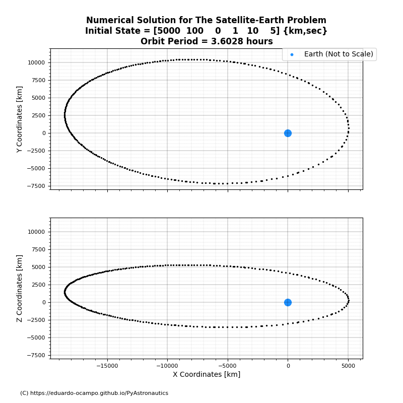
To illustrate the numerical results, the satellite’s trajectory is projected on the x-y & x-z plane as shown in Figure 1.2

Figure 1.2 Satellite Trajectory Projected on 2D Planes

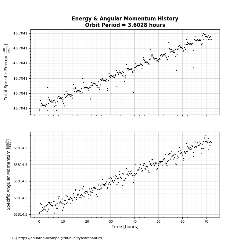
It is good practice to spot check the results by checking if Specific Energy (\(\varepsilon\)) and Specific Angular Momentum (\(h\)) are conserved throughout flight. Figure 1.3 shows both \(\varepsilon\) & \(h\) as a function of time. As we expect the characteristic parameters are conserved. The slight increase over time is due to computation limitation but take note of the y-axis range.

Figure 1.3 History of Energy and Angular Momentum Parameters

Lastly, a 3-dimensional plot of the satellite’s trajectory is shown below in interactive Figure 1.4.

Figure 1.4.

Play the animation by pressing the blue button and rotate the figure using your mouse. The duration (Time of Flight) of the animation is equivalent to 1 orbital period. Notice how the satellite’s relative speed compares at periapsis and apoapsis. At periapsis, the satellite’s altitude is 4,926.081 km and its relative speed is 2.94710 \(\frac{\text{km}}{\text{s}}\) while at apoapsis the altitude is 18,938.773 km and at a speed of 1.33245 \(\frac{\text{km}}{\text{s}}\).

This example is a quick walk through on how to use module astrodynamics.two_body_problem. There are more uses for the Two-Body Problem solution that is left for the reader to explore. Below is one last example of generating the spacecraft’s orbital anomalies using the solution to the initial value problem:

# Calculate True Anomaly History
e = self.orbit_elements.e_vector.value
f = [np.arccos(np.dot(e,p) / 
                (norm(e)*norm(p))) 
                for p in self.numerical_position]

self.orbit_elements.add_parameter("f",
                                    np.degrees(f), "degrees",
                                    description="True Anomaly")