CR3BP Python Example

Using the equations of motions derived in the Non-Dimensional Circular Restricted Three-Body Problem (CR3BP) section let’s walk through a simple example of solving for the trajectory of a spacecraft along the Earth-Moon system.

Problem Definition

Boundary Conditions

In the rotating frame the non-dimensional initial position and velocity vectors are given as:

(1)\[\begin{split}\mathbf{r}^*(t_0) = \begin{bmatrix} 0.50 \\ 0.50 \\ 0.00 \end{bmatrix}\end{split}\]

\[\begin{split}\mathbf{v}^*(t_0) = \begin{bmatrix} -0.05 \\ 0.10 \\ 0.00 \end{bmatrix}\end{split}\]

The Earth-Moon mass ratio is:

\[\mu = 0.012150515586657583\]

Differential Equations

The numerical solver relies on running scipy.integrate.solve_ivp() to solve the initial value problem for the system of non-dimensional (6) ordinary differential equations.

\[\begin{split}\begin{align*} \ddot{x}^* - 2\dot{y}^* &= \frac{\partial{\tilde{\mathbf{V}}}}{\partial{x^*}} \\ \ddot{y}^* + 2\dot{x}^* &= \frac{\partial{\tilde{\mathbf{V}}}}{\partial{y^*}} \\ \ddot{z}^* &= \frac{\partial{\tilde{\mathbf{V}}}}{\partial{z^*}} \end{align*}\end{split}\]

When taking the partial derivate of \(\tilde{V}\) or \(\tilde{U}\) the distance vector \(\mathbf{r^*}\) is a function of time and must be decomposed in the process.

(2)\[\begin{split}\mathbf{\dot{r}}^* = \begin{bmatrix} v^*_x\\ v^*_y \\ v^*_z \end{bmatrix}\end{split}\]

(3)\[\begin{split}\mathbf{\ddot{r}}^* = \begin{bmatrix} 2v_y + x - \frac{\left(1-\mu\right)\left(x+\mu \right)}{{r^*_1}^3} - \frac{\mu\left(x + \mu -1\right)}{{r^*_2}^3}\\ -2v_x + y\left[1 - \frac{1-\mu}{{r^*_1}^3} - \frac{\mu}{{r^*_2}^3}\right] \\ -z \left[ \frac{1-\mu}{{r^*_1}^3} + \frac{\mu}{{r^*_2}^3} \right] \end{bmatrix}\end{split}\]

Python Setup

Now begin by importing Python class CR3BP() from module astrodynamics.three_body_problem or from astrodynamics directly as shown below:

from pyastronautics.astrodynamics import CR3BP

and define the initial state vector using the given initial boundary condition (1):

initial_position = [0.50, 0.50, 0.0]
initial_velocity = [-0.05, 0.10, 0.0]

Instantiate class CR3BP() with the initial state vector and set the mass ratio \(\mu\) for the analysis of a spacecraft (sc) within the Earth-Moon system.

# Earth-Moon Mass Ratio
mu = 0.012150515586657583

sc = CR3BP(initial_position,initial_velocity)
sc.mu = mu

For this example, the interval of integration will be set to non-dimensional time of \(8\pi\).

\[t_f = 8\pi\]

time_num = 1000
sc.time = np.linspace(0, 2*np.pi*4, time_num)

Solve for the spacecraft trajectory over time \(t_f\). By flagging the argument save_analysis = True the numerical solution is saved off as a pickle file. Allowing for the user to solve a complex initial value problem only once and loading the results later for post-processing. By default the solution will be saved as cr3bp_solution.pickle but this can be changed by renaming attribute CR3BP.num_sol_pickle_file to the desired file name.

sc.solve_non_dim_trajectory(save_analysis=True)

The numerical results are available by accessing sc.num_sol, For convenience the position and velocity over time of flight are store as sc.numerical_position and sc.numerical_velocity.

results = sc.num_sol

numerical_position = sc.numerical_position
numerical_velocity = sc.numerical_velocity

Results

Plotting the results shows the spacecraft’s trajectory for a non-dimensional time of \(8\pi\). It appears to be stable while orbiting the Earth at some periodic rate. To better illustrate the time of flight a blue gradient trajectory is plotted along non-dimensional axes showing where the spacecraft started and ended along the Earth-Moon system.

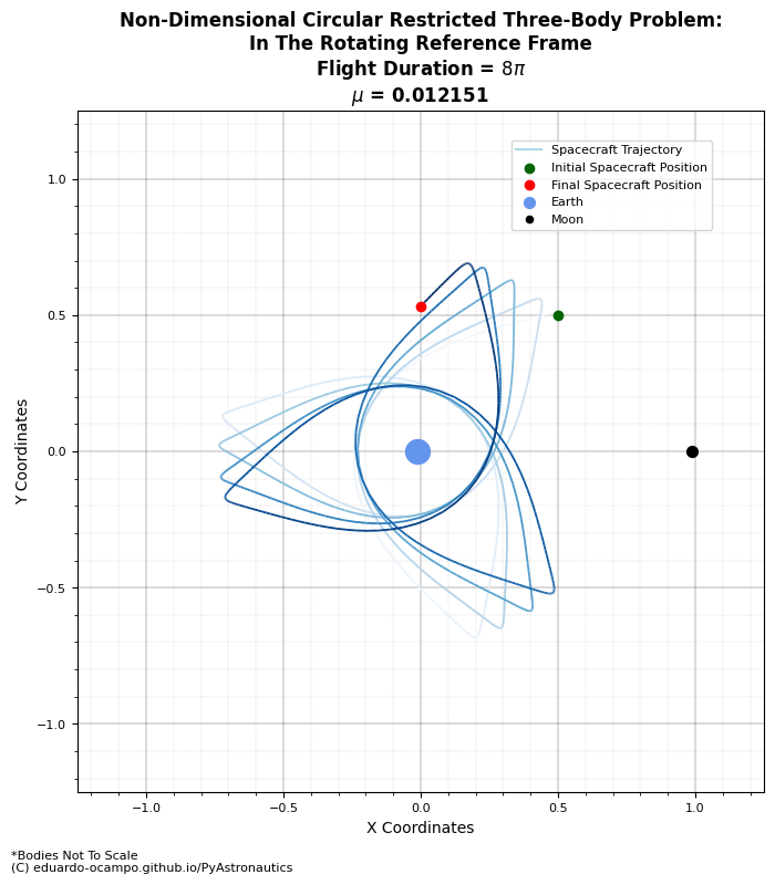
Figure 1.7 Example Solution to the CR3BP in the Rotating Reference Frame

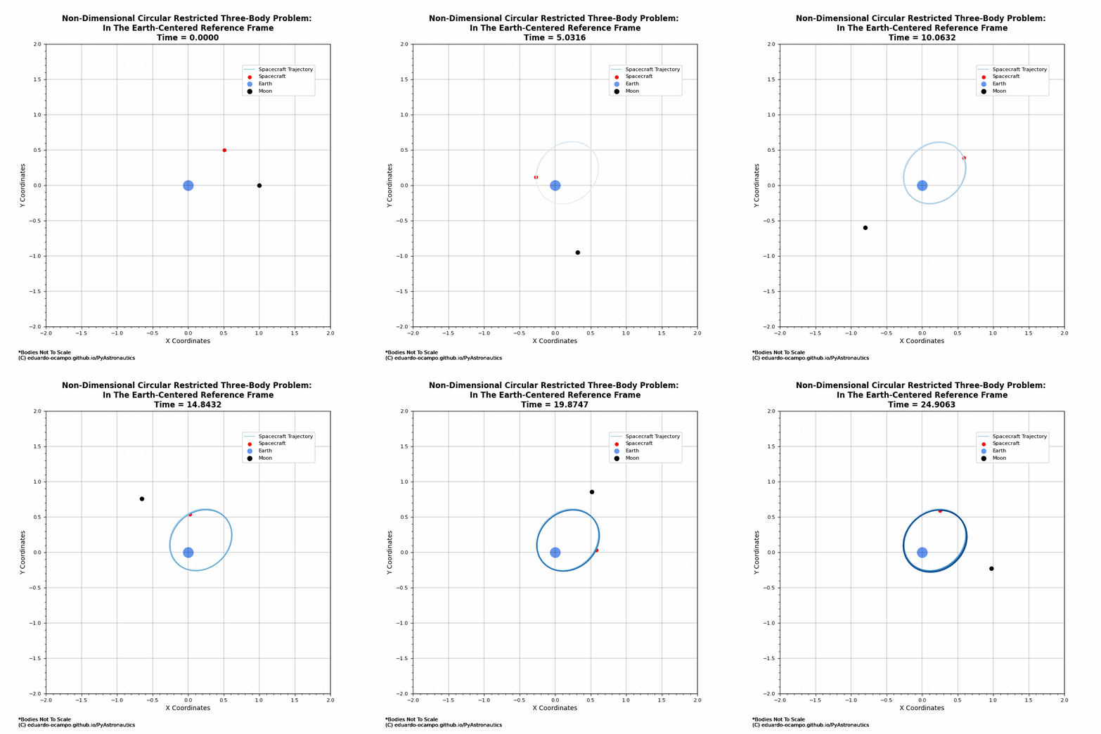
Figure 1.8 Animated Trajectory of the CR3BP Example in the Earth-Centered Frame

Moon Orbit Transfer

There are natural pathways from Earth’s orbit to the Moon for better fuel efficiency using the third body effects. To motivate why we should study the Three-Body Problem I will provide some examples of “cheaper” ways to the moon.

This example starts with a spacecraft in Earth’s orbit at some initial position and velocity. Assume prior to this initial state, the spacecraft was at some geostationary orbit and some \(\Delta V\) was applied to get it to \(\mathbf{r}^*\), \(\mathbf{v}^*\):

\[\begin{split}\mathbf{r}^*(t_0) = \begin{bmatrix} 0.50 \\ 0.50 \\ 0.00 \end{bmatrix}\end{split}\]

\[\begin{split}\mathbf{v}^*(t_0) = \begin{bmatrix} 0.0998780 \\ 0.5941623 \\ 0.00 \end{bmatrix}\end{split}\]

Solution

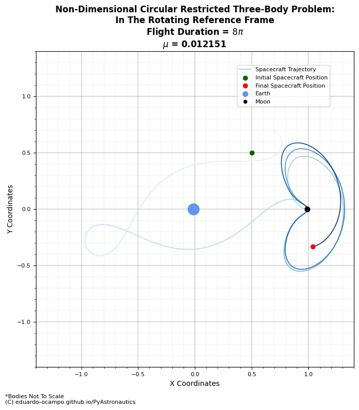
Figure 1.9 Example of The Moon’s Orbital Influence

Figure 1.10 Animated Trajectory of The Moon’s Orbital Influence

As shown in the animation, the first past by the Moon the spacecraft got a bit of a nudge which increases its orbital perigee. After which it is in a loose lunar orbit as illustrated better in the rotating frame (Figure 1.9).

Moon Capture

Part of the art of setting up a “cheaper” path to the Moon is lining up the phasing of the Moon and spacecraft’s trajectory. When done correctly the spacecraft will naturally get captured by the Moon with the right \(\Delta V\). Here is a better example from a new initial state:

\[\begin{split}\mathbf{r}^*(t_0) = \begin{bmatrix} 0.00 \\ -0.50 \\ 0.00 \end{bmatrix}\end{split}\]

\[\begin{split}\mathbf{v}^*(t_0) = \begin{bmatrix} 0.8733718532917388 \\ -0.5247747524101218 \\ 0.00 \end{bmatrix}\end{split}\]

Solution

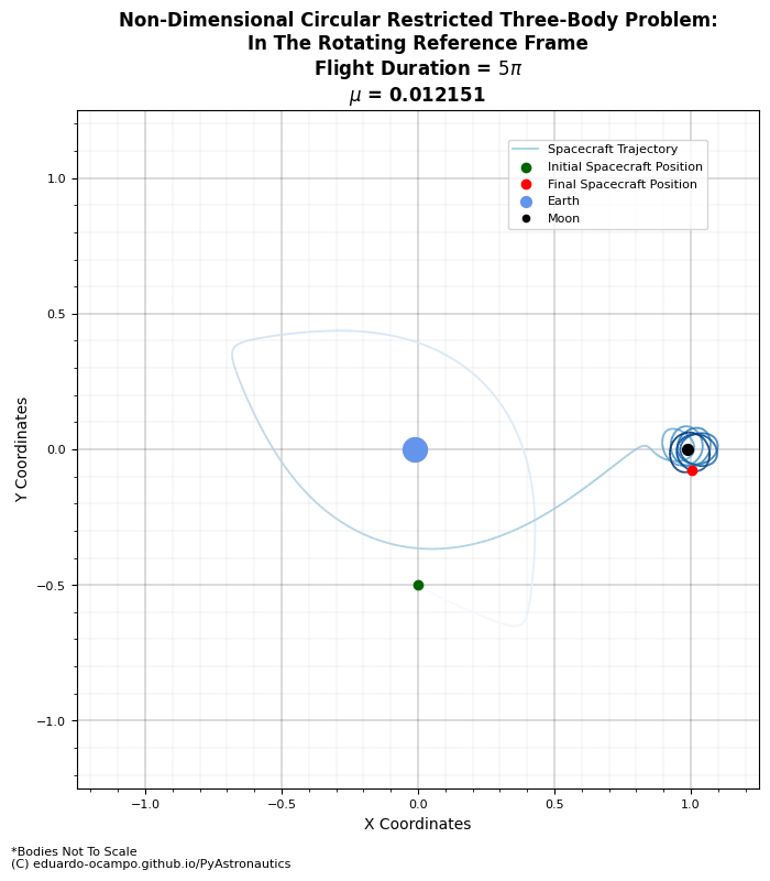
Figure 1.11 Example of Moon Orbit Transfer

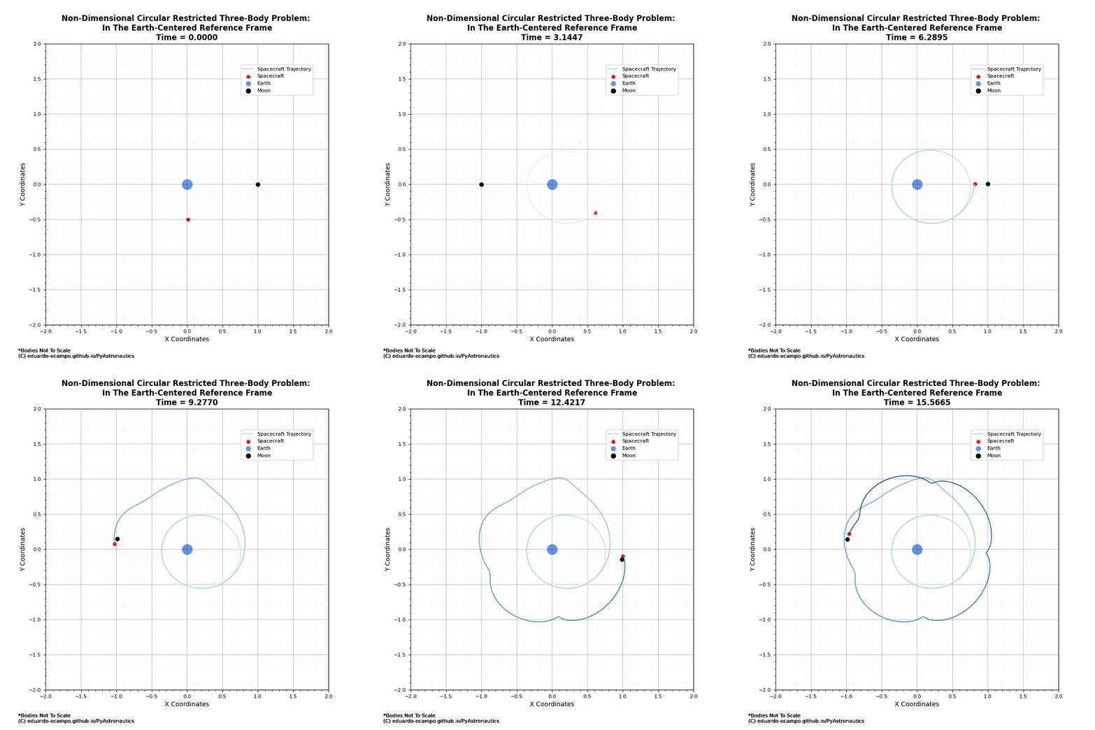
Figure 1.12 Animated Trajectory of Moon Orbit Transfer