Circular Planar Restricted Three-Body Problem¶

For a simplified solar system, the motion of the planets are more or less in the ecliptic plane. Often times it is not a bad approximation to assume that \(z\) and \(\dot{z}\) are to be zero (small inclination).

\[\frac{d\mathbf{\tilde{V}}}{dt}\bigg|_{z^* = 0} = 0\]

In other words, we can decouple the in-plane motion and out-of-plane motion. This system is named the Circular Planar Restricted Three-Body Problem (CPR3BP). In this case Non-Dimensional Jacobi Constant (5) simplifies to:

(1)¶\[\left( {\dot{x}^*}^2 + {\dot{y}^*}^2\right) - 2\tilde{V}\left(x^*,y^*\right) = 2\tilde{J} = -C\]

A new constant ( \(C\) ) is used to denote the Circular Planar Restricted Three-Body Problem Jacobi Constant.

The form of the Jacobi Constant is similar to that of total energy such that it has a pseudo-potential term and a kinetic energy like term. Understanding Jacobi constant gives insight to a spacecraft’s motion in the Three-Body System and its limits in space.

Looking at the velocity term in Equation (1) it is certain to always be positive. Rearranging Expression (1) shows that \(2\tilde{V} - C \ge 0\).

Knowing \(\tilde{V}\) is always positive, if \(C \lt 0\) then \(2\tilde{V} - C \ge 0\) is always satisfied. However, if \(C \gt 0\) things get a bit interesting. This says for a given value of Jacobi Constant, motion is not possible in the region of space when:

(2)¶\[2\tilde{V} - C \le 0\]

In Astrodynamics the curve in space where the velocity would go to zero is referred to as Zero-Velocity Curves or Forbidden Regions. For the CPR3BP the Zero-Velocity Surface is defined as:

(3)¶\[2\tilde{V}\left( x^*, y^*\right) - C = 0\]

The next section will dive into generating Forbidden Regions of space using Python.

Forbidden Regions¶

Consider the Earth-Moon System. The Planetary Satellite Mean Elements are pulled from Solar System Dynamics database courtesy of NASA JPL.

Planet	Satellite	Code	Ephemeris	a (km)	e	ω (deg)	M (deg)	i (deg)	node (deg)	P (days)
Earth	Moon	301	DE405/LE405	384400	0.0554	318.15	135.27	5.16	125.08	27.322

With the Moon’s inclination of 5.16\(^\circ\) the Circular Restricted Planar assumption is valid for this analysis.

The following constants were generated for the Earth-Moon system using NASA JPL’s Solar System Dynamics Astrodynamic Parameters database (\(\frac{km^3}{s^2}\)):

\[\begin{split}\begin{align*} GM_{\text{Earth}} &= 398600.435507 \\ GM_{\text{Moon}} &= 4902.800118 \\ \end{align*}\end{split}\]

Yielding a mass ratio of:

\[\mu = 0.012150584394709708\]

For this example, plot the forbidden regions for the CPR3BP at Jacobi Constants ranging from 3.5 to 3.0. Here the Lagrange Points are plotted for reference as they are relevant to the forbidden regions. More information about the Lagrange Points can be found here.

Begin by importing class CR3BP from module astrodynamics and defining the Earth-Moon mass ratio \(\mu\).

from pyastronautics.astrodynamics import CR3BP

# Earth-Moon System Parameters
# ----------------------------------------------------------
mu = 0.012150584394709708

Function CR3BP.forbidden_region() can be used to compute the forbidden region in the x-y plane based on the Jacobi constant and mass ratio.

# Calc Forbidden Region
# ----------------------------------------------------------
# meshgrid spacing
lin_num = 150

# Jacobi Constant
C = 3.5

# Get Forbidden Region
x1, y1, forb_region1 = CR3BP.forbidden_region(C,mu,linspace_num=lin_num)
x2, y2, forb_region2 = CR3BP.forbidden_region(C,mu,linspace_num=lin_num,
                                              x_range=[ 0.70,1.20],
                                              y_range=[-0.25,0.25])

It has x-y coordinate ranges set by default but in some cases they may be set by the user. Argument linspace_num is used to set the density of the meshed grid used for building the forbidden region. This example sets a coarse np.linspace spacing for easier to load interactive figures included in this section.

Using this method, interactive Figure 1.13 was created to draw forbidden region contours for 8 Jacobi Constant (\(C\)) values for the Earth-Moon system. Move the slider at the bottom of Figure 1.13 to view the different contour plots.

Figure 1.13. Interactive Forbidden Region Contour Plots

Figure 1.13 is initialized with slider set to \(C = 3.5\) for reference. As the Jacobi Constant for the Earth-Moon System decreases towards 3.0 notice how the forbidden region gets smaller in size.

As Jacobi Constant \(C\) continues to decrease in Figure 1.13 the region in space between both Lagrange Point 2 and Lagrange Point 3 begin to open. This is shown in Figure 1.13 by toggling slider between \(C = 3.180\) and \(C = 3.013\). As \(C\) gets closer to 3.0 the forbidden regions disappear to a singularity corresponding to the location of Lagrange Point 4 (L4) and Lagrange Point 5 (L5). For the Earth-Moon System the minimum Jacobi Constant is approximately 2.988043. This can be shown by hovering your cursor around L4 and L5 on interactive Figure 1.13.

For \(C = 3.18827\) the forbidden region around the Moon comes to a singularity at Lagrange Point 1. As shown with more detail in Figure 1.14 below.

Figure 1.14. Singularity of the Jacobi Constant at L1

Now for \(C \lt 3.18827\) a direct path from the Earth to the Moon begins to appear (Low Energy Transfer). At a high level, Mission Design Engineers aim to change a spacecraft’s velocity just enough so that a trajectory exists between two primary bodies using very small energy. For example, here are some more references for how this is used on the Earth-Moon system for Low Energy Transfer and Free-Return Trajectory as means of sending spacecraft to the Moon.

Using the static function CR3BP.get_jacobi_velocity() provided in module astrodynamics one can get the required maximum velocity for a given Jacobi Constant. Let’s use this function to determine the velocity required to transfer from an Earth parking orbit to the Moon’s region in space at initial position and a fixed velocity angle \(\theta_0\):

(4)¶\[\theta_0 = 31^\circ\]

(5)¶\[\begin{split}\mathbf{r_0}^* = \begin{bmatrix} 0.00 \\ -0.50 \\ 0.00 \end{bmatrix}\end{split}\]

Import class CR3BP and set the initial state vector for this example using get_jacobi_velocity.

from pyastronautics.astrodynamics import CR3BP

# Initial State Vectors
# --------------------------------------------------------------------------------
initial_angle = np.radians(31)
x_initial, y_initial =  0.00, -0.5
vel_initial = CR3BP.get_jacobi_velocity(x_initial,y_initial,C,mu)

initial_pos = [x_initial, y_initial, 0.0]
initial_vel = [ np.cos(initial_angle)*vel_initial, 
                -np.sin(initial_angle)*vel_initial, 0.0]

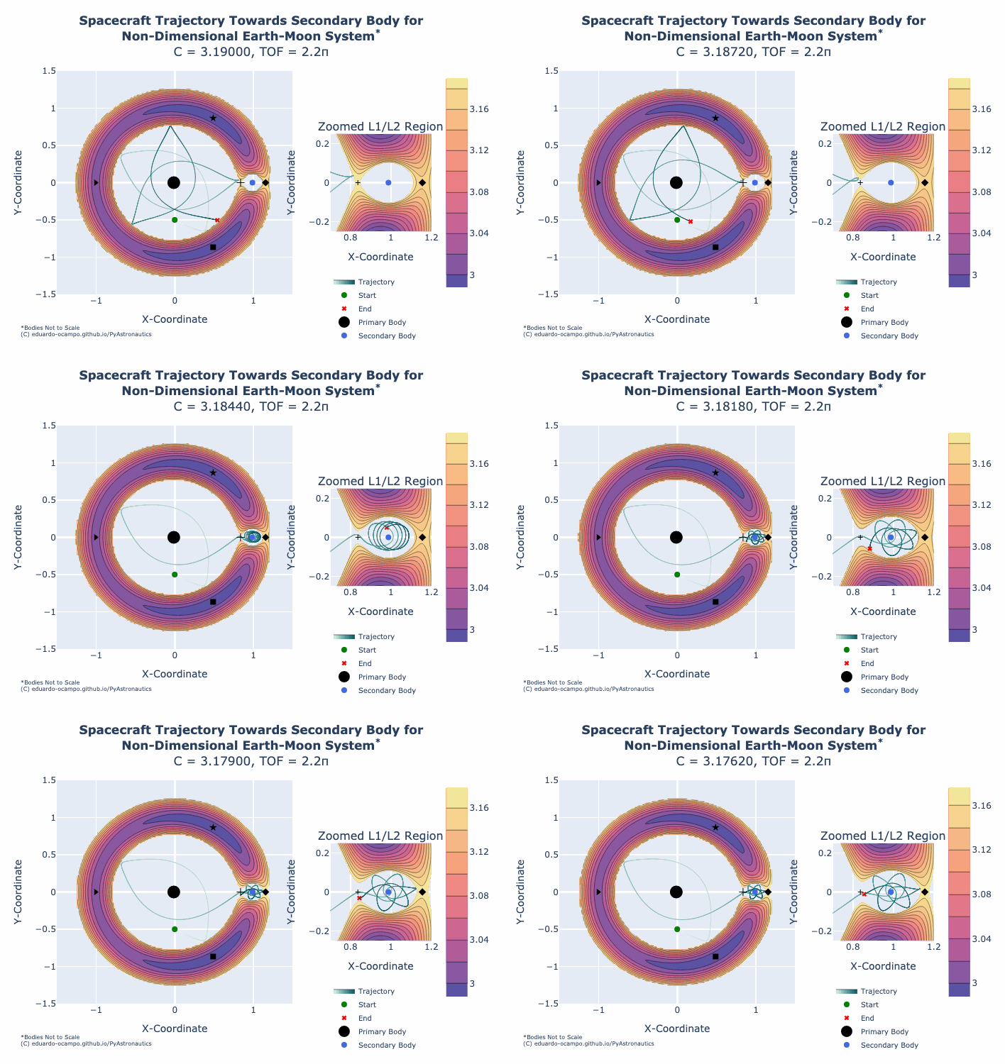
Use the same methods from Python Example for generating a trajectory in the Non-Dimensional Circular Restricted Three-Body Problem to show the interaction between a spacecraft’s change in energy and the Jacobi Constant:

../../_images/moon_region_trajectory.gif — **Figure 1.15** Animation of Trajectory Towards the Moon¶

The animation shows the Jacobi Constant starting at a value of 3.190 and ending with a constant of 3.176. For a fixed spacecraft position (5) and impulse angle (4) as \(C\) decreases the magnitude of \(\Delta V\) required to maintain the Zero-Velocity Surface (3) increases from 1.015956 to 1.022823. If the mission requirements is to design a trajectory towards the Moon region of space, than we can analyze the minimum \(\Delta V\) required until the L1 region opens up but notice how the orbit shape around the Moon also changes with increased velocity. At some point the increase to the initial velocity sets the spacecraft up to return towards L1 and given a \(TOF\gt 2.2\pi\) the spacecraft can return towards the primary body.

Zero-Velocity Curves¶

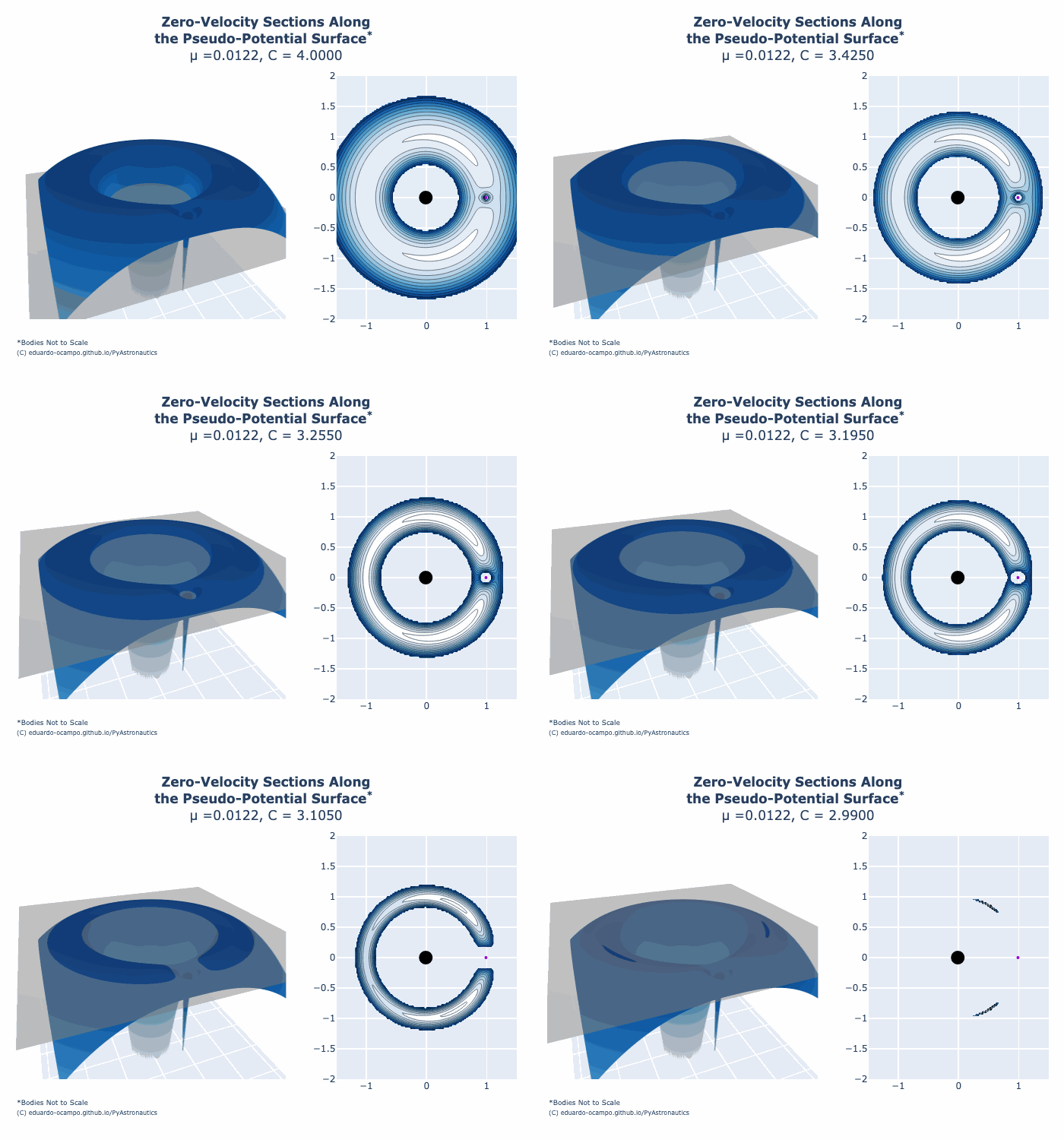
Lastly, the same analysis can be done to demonstrate how the forbidden regions change in 3-dimensional space along the Potential Surfaces (7) introduced in section Non-Dimensional Circular Restricted Three-Body Problem

../../_images/zvc_cross_section.gif — **Figure 1.16** Animation of Zero-Velocity Curves for the Earth-Moon System¶

Acknowledgements¶

Special thanks to Ari Rubinsztejn of gereshes.com for their publication on the Three-Body Problem. Their work played a key role in helping verify & validate the Python routines I created for this section. I encourage the reader to visit Rubinsztejn’s work on the Jacobi Integral and how it varies with \(\mu\), or at the very least appreciate the informative plots they created by visiting their site Jacobi and His Constant – The 3-Body Problem.